Context
One of the primary goals of this project was to explore the possibilities surrounding modeling a custom-built aircraft. In the long term I will work to answer the following questions:
- Can parameters accurately be estimated exclusively from flight data?
- Can these parameters be entered as states in the filter and changed during flight? (see more details in post on Simultaneous State and Parameter Estimation)
- If so how many can be changed at once?
- Could these parameters be able to change fast enough to adapt to a model major change in the system (loss of wing or shift of CG)?
- Could a model-based control system use the changing parameters to adapt the control scheme? (This bleeds into the actual field of adaptive control which will be involved in the future)
For this post, I'm going to simply focus on this first bullet point.
Aircraft Model
Aircraft modeling is notoriously difficult and complicated to the point that many aspects are still ongoing sources of research. Therefore the decision I had to make when selecting a model is not whether or not to generate a perfect model but instead find what approximations are reasonable to take for now. After searching around for a while, I settled on the model used in Cornell's Flight Dynamics course, full pdf here. This source does a great job of deriving the relevant coefficients and displays the linearized, decoupled, state-space results in section 5.2. Assuming that the aircraft naturally flies close to level (a valid assumption given the attitude data from the most recent flight), the state-space model looks like this:

Here, $u_0$ is the steady-state velocity, $\Theta_0$ is the steady-state angle of attack, which we're already assuming is 0, and the $\delta$ terms are the control surfaces. Also, note that all state and input terms are $\Delta$s meaning that they are the difference of the state from the steady-state, or equilibrium, value.
There are a few major assumptions in this model. The first is linearity. All dynamics have been linearized about level flight. For this reason, when recording data, I tried to fly casually and maintain an attitude that would validate this assumption. The second assumption was that the roll and pitch axes are independent. This assumption is clearly not true in reality because at any bank angle or pitch angle many basic physics and aerodynamic effects cause mixing, but given the small-angle linearity assumption, the off-axis motion effects become negligible in comparison to the effects of the on-axis motion.
You'll also notice that these parameters don't resemble the coefficients of lift, drag, or moment that aerodynamics students are familiar with. This is because each parameter is a combination of all relevant terms as well as the mass and moments of the aircraft. The beauty behind working at this high level is that the estimator does not need to know what goes into the parameters, only how they act. In addition, once these parameters have been estimated, the equations can be inverted to derive the original coefficient equations.
Mathematical Process
In order to actually find these coefficients, I first had to pull every $\Delta$ state and input term present in the dynamics equation from the flight data. This required either finding or defining an equilibrium value and taking the difference at every step. It also required finding the finite difference derivative of each state at every step.
All states except for forward velocity, $u$, were assumed to have an equilibrium value of 0. This is consistent with the level flight assumption from earlier. To find $u_0$, equilibrium of $u$, I found the mean $u$ during normal flight.

The equilibrium values for the servos were found empirically through tuning the aircraft in flight. Since the trim switches on the transmitter allow for minor adjustment of the servo middle, I was able to trim the control surfaces so that the aircraft flew level with no input. These values were used as the equilibrium for the control surfaces.
On the topic of control surfaces, we arrive at another assumption. So far, I've been recording servo inputs as the angle sent to the servo. However, there is a linkage between the servo and the actual control surface causing a non-linear conversion (Freudenstein Equation is the true mapping) between the control surface and servo. However, since we are using arbitrary parameters to convert from control surface throw to dynamics derivative, the unit conversion and necessary factors can be swallowed into the parameter term as long as the relationship can be assumed as linear. For the specific setup used here, that was a reasonable assumption.
If we convert the dynamics equations into their matrix state-space representations, $\dot{\textbf{x}} = A \textbf{x} + B \textbf{u}$, we have recorded vectors for every state of $\dot{\textbf{x}}$, $\textbf{x}$, and $\textbf{u}$. In order to compute the best estimate value for every value in the A and B matrices, we can compute the least-squares fit of every row of A and B to find an estimate of each. This requires a bit of rearrangement, especially where there are constant values like the gravity term in the first rows of both pitch and roll, but eventually, every row can be converted to the following form:
$$y = \Theta x$$
where $y$ holds the state derivative terms, $x$ holds the state and input terms, and $\Theta$ holds the parameter vector specific to each row. The least-squares optimal value for each $\Theta$ is defined as
$$ \hat{\Theta}=yx^T(xx^T)^{-1}$$
By computing this for each unknown parameter, I generated an approximate state-space model for the aircraft.
Examining Results
Pitch Direction
Though it would be difficult to verify the predicted state-space models without more data, we can look at their eigenvalues and simulated behavior and compare it to what is expected from aircraft dynamics.
We first examine the eigenvectors of the open loop system:
$$ \lambda_1 = -32.1592 + 0.0000i $$
$$ \lambda_2 = -7.2258 + 0.0000i $$
$$ \lambda_3 = -0.1275 + 0.5557i $$
$$ \lambda_4 = -0.1275 - 0.5557i $$
Here we see one set of complex eigenvalues and two negative real eigenvalues. For large aircraft, it is expected to see two sets of complex eigenvalues representing the short period and phugoid modes. Here, we are only seeing one. I expect that this one is the phugoid mode because the phugoid mode is slightly damped and is largely independent of vehicle parameters suggesting that it would show up regardless of the vehicle size. We can verify this by looking at its simulated behavior with an initial pitch-up angle.

This mode has the corresponding period: $T=11.3059$s. This long time scale period and lightly damped oscillation confirm that what we are seeing is the phugoid mode.
There are a lot of potential explanations for why there is no short period mode. The frequency of my data collection might not be fast enough to see it? There might not be enough data for it to show up consistently? It was not properly excited by this flight? There is a bug in my code? Or maybe the short period mode does not show up on this aircraft? A foamboard plane is a far cry from a 747 after all. For now, I will be satisfied with the phugoid mode. It is much less damped anyway and so much more important to control.
For some more basic sanity checks, we can observe from the above plot that the increase in velocity caused the vehicle to pitch up which in turn slowed the vehicle down, pitching it down and speeding it up again. This is expected behavior.
Elevator
If we add in some positive elevator at 5 seconds, we see the aircraft pitch up and slow down, again, as expected.

Up Elevator added briefly at 5 seconds
Throttle
For an increase in throttle at 5 seconds we see the forward velocity increase linearly which makes physics sense. In addition, we see the aircraft pitch forward. This also makes sense and is a result of the pusher prop's thrust line crossing above the center of mass and adding a forward moment.
Positive throttle added briefly at 5 seconds
Roll Direction
In the roll direction we expect to see one damped oscillatory mode and two damped exponential modes. The damped oscillatory mode is called the Dutch roll mode and comes from the combined effect of rolling, slipping and yawing. The eigenvalues of the estimate parameters are below:
$$ \lambda_1 = -36.0670 + 0.0000i$$
$$ \lambda_2 = -20.2693 + 0.0000i$$
$$ \lambda_3 = -0.3128 + 0.4873i$$
$$ \lambda_4 = -0.3128 - 0.4873i$$
As anticipated (or at least as I hoped), we see one lightly damped oscillatory mode and two heavily damped exponential modes. The period on this oscillatory mode is 12.894s.
To further sanity check the behavior we run the following tests.
First, we give the initial roll angle a slightly positive rate. This is equivalent to banking right.

Initial positive $\phi$ angle
As expected, the initial condition is quickly dampened with some small oscillation. While the angle was positive, the $\Delta v$ term was also positive, showing that the right bank caused some rightward velocity. This is again expected and encouraging.
Aileron
When we apply a slight rightward rolling aileron actuation at 10 seconds we see below that the rate immediately spikes and the aircraft rolls about the x-axis to the right, both as expected. However, what's far more interesting and got me more excited is the effect that the roll has on yaw. You see here that a rightward roll causes a negative rate about the yaw axis. Since the yaw axis points down, this negative rate causes the aircraft to yaw away from the roll direction. This is known as adverse yaw and is a much finer detail behavior than I expected to find from this data.

Right rolling aileron actuation at 10s
Rudder
By giving a little bit of right rudder at 10 seconds, we see that, as expected, the rate about the phi axis increases, and the aircraft rotates right. The more interesting result is that the roll axis also pitches slightly right. The reason for this is that the aircraft has some minor dihedral for stability. That means that when you yaw one direction, you also roll that way too. This is actually how a 3 channel aircraft flies. I am again surprised and excited to see this behavior show up in the data.
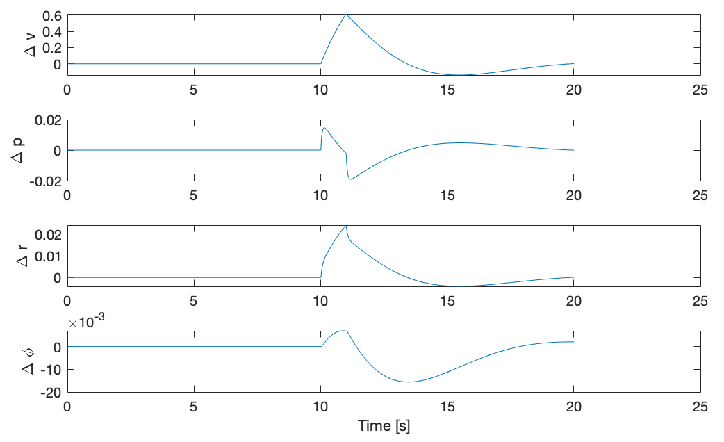
Righr rudder applied briefly at 10s
Conclusions and Future Steps
I want to first off say how excited I am to be getting these results. Everything I described doing in this post was something that I came up with and wanted to try with very few references or prior examples. There were so many places that this could go wrong between the hardware, onboard software, filter, aircraft, and the parameterizing that I am truly overjoyed to be seeing so many behaviors that I associate with my exact aircraft.
This now opens the flood gates to so many future steps. With a reasonable model, I can now begin to design a truly model-based control system. I will start with LQR due to the multi-input, multi-output nature of my state-space model. I can also apply this model to a Model-Based estimator and make actual prediction steps. This should improve my state estimates even more and allow me to make better estimates of my parameters. The final step I can now take is to begin to experiment with the idea that started all of this. What happens when I make every one of these parameters a state in my filter? Can I be getting better and better estimates throughout the flight? I'm very excited. I hope you are too. Please stick around.


No comments:
Post a Comment