Initial Controller Design

Overview

Before adding the controller to the onboard software, I had to design it in simulation. Fortunately, I had now an approximate model to use for design. In this post, I'll go over the process of designing a model-based controller in simulation.

Constraints

Since I'll be designing this control in simulation but planning to use it on an actual system, there are a few things that the simulation won't show me that I need to keep in mind. The first of these is the actual limitation of my actuation. My servos are real objects and therefore have limited range, speed, and acceleration. I've documented the expected range of the servos on my aircraft. Dealing with speed and acceleration is more difficult. Unfortunately, I cannot find the datasheets for the servos I'm using. Even if I did, the acceleration, in particular, would change in flight due to the aerodynamic load. To solve this, I am going to find the max speed from a weaker servo that I can find the datasheet for and use its limitation as a conservative estimate for my own servo. Within the simulation, I will cap the servo's output speed to this max speed so that non-physical servo motion is not simulated.

I initially was using MATLAB's lsim to simulate the motion. However, there is no method to access the control input in a closed-loop system with lsim so I ended up writing my own function to replace lsim with my own functionality.

Expected Perturbations

In order to test the control response, I first need to perturb the system. I would like to perturb the system with realistic forces and torques. This is the same as finding the expected process noise of the system. Fortunately, this is very simple using the same math and code I'd set up previously to generate the parameter estimates.

The estimates were fit to find the best estimate for the equation $y=\Theta x$ for every row of the state space matrix representation where $y$ is 1xn the vector of state derivatives, $\Theta$ is the 1xm parameter vector, $x$ is the mxn state and controls vector, n is the number of data points, and m is the number of parameters. Since $y\neq\Theta x$ for any specific data point, the residual $y-\hat{\Theta} x$ contains the process noise vector for the flight.

The mean and standard deviation of these vectors both interest me. Below are the calculated values after non-physical outliers were removed:

$$\Delta\dot{u}: \text{Mean}:   0.9327m/s^2    1\sigma:  12.1979  m/s^2$$

$$\Delta\dot{v}: \text{Mean}:   -3.6895m/s^2   1\sigma:  13.5130   m/s^2$$

$$\Delta\dot{w}: \text{Mean}:   2.4308m/s^2   \text 1\sigma:  30.9169  m/s^2$$

$$\Delta\dot{p}: \text{Mean}:   2.3433rad/s^2   \text 1\sigma:   13.1695  rad/s^2$$

$$\Delta\dot{q}: \text{Mean}:   6.6781 rad/s^2   \text 1\sigma:  35.6544   rad/s^2$$

$$\Delta\dot{r}: \text{Mean}:   -2.0239rad/s^2   \text 1\sigma:  24.4184   rad/s^2$$

My first reaction to all of these numbers is that they seem very large. Though instantaneous acceleration is a more difficult thing to have a gut feel for than velocity or distance, I'm still surprised that the 1 sigmas for acceleration are over a 1g, 3g for the case of the direction of gravity. The rotation rates also feel very high. 

There are a number of explanations. The first is that I do not have a feel for the forces and torques that foamboard aircraft feels in the sky and so my instinct is incorrect. In addition, the process noise accounts for the differences between the nonlinear truth and linear model, so some of the error could be from the approximation. There also might have been significantly more wind up high than I expected. And of course, there could be a bug in my code.  For now, I will move forward with these values and see what kind of controller it takes to null them out.

Design Choice and Simulated Runs

We will do the initial design by perturbing the initial state vector and examining the controller's response. For initial perturbations, I will use the mean and $1\sigma$ values from the process noise to generate an initial state error using the following equation.

$$\Delta x_0=(\text{mean}+1\sigma)\times0.1$$

0.1 is a relatively rough number that I'm using but I don't think it will matter too much because after studying the effects of initial state perturbations, I will move onto constant force perturbations. These should be more accurate anyway.

For the controller itself, I will be starting with an LQR designed state-space controller. This optimal controller works very well for multi-input multi-output models like this one. I will begin by designing in continuous time. Though the actual implementation will be running in discrete time, the 20Hz operating frequency is significantly faster than the modes of the system (see periods for oscillation of modes from the last post), so I believe it is reasonable to design in continuous time without too much adjustment for discrete-time. This is another assumption that I will check the validity of through flights and return to if invalid.

Pitch

The controller I settled on for pitch weighted the velocities v, and w, the same, with the pitch rate being 10x less important and the pitch angle 10x higher. This was all weighted as 500x higher than the control inputs. 

$$Q= 500\times\textbf{diag(}[\  1\  1/100\  1\  10\  ]\textbf{)}$$

$$R= \textbf{diag(}[\  1\  1\  ]\textbf{)}$$

In response to the initial perturbation, $[1.31\  3.33\  5.38\  0]$, the response was as shown below.

Pitch response to initial condition perturbation

As shown, all states are within 10% of their original values after 5 seconds. In addition, the controller and elevator inputs are relatively small. For reference, there are over 80 degrees of deflection available to both the throttle and elevator in both directions.

In a slightly more interesting example, the system is given a constant force equal to the bias in the $u$ state. The difference here is that the error is not in the initial condition but instead in a constant acceleration/torque vector applied to the state.

Perturbed with constant force in $u$ direction

The aircraft pitches up and then achieves a new steady-state state and control inputs. You'll also notice an interesting behavior where the Throttle and Elevator work in tandem. Because the throttle pitches the aircraft forward when the throttle increases, the elevator goes up and vice versa.

With some noise added, the results are similar to the above, though no true steady-state is reached due to the constant noise.

Perturbed with constant force and noise in $u$ direction

It is worth noting that even though I've capped the max speed of the servos to a reasonable value, I haven't capped the servo acceleration so it is possible that the quick and fine adjustments aren't possible. There are ways that I can increase the fidelity of this model to truly account for the servo's capability but I believe that this too detailed for this type of simulation and I would rather spend time on other aspects for now.

Roll

I specified the weights for the roll axis very similarly to the pitch axis, with a little bit of extra tuning. I settled on the rotations rates being 100x smaller than the $v$ velocity and the angle $\phi$ being 10x higher. The velocity was also 100x higher weighted than the control inputs. 

$$Q= 100\times\textbf{diag(}[\  1\  1/100\  1/100\  10\  ]\textbf{)}$$

$$R= \textbf{diag(}[\  1\  1\  ]\textbf{)}$$

The response to the initial state perturbation, calculated the same as for pitch, is shown below.

Roll response to the initial state perturbation

All states are nulled to 10% of their max values within 1 second. In addition, the control outputs are both of similar order of magnitude to what we saw in the pitch axis. This is very reasonable and attainable for the physical system.

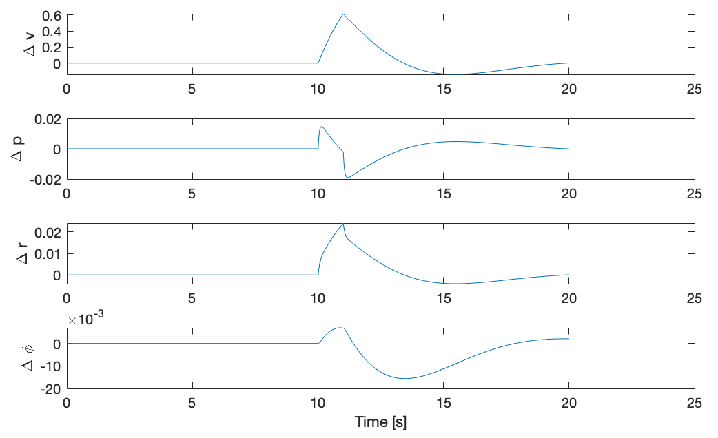
We can look at a more realistic case by adding both the bias and random noise with the same distribution as found from the residuals. This has the following response.

Here we see that the open-loop angle and velocity arrive at large final offset values but the controller manages to keep both states below 20% of their open-loop error. In addition, we notice that the rates of both open loop and closed loop $r$ and $p$ are very similar. This is a combination of the rotational acceleration being directly connected to the process noise and the controller prioritizing the angle and velocity over angular rates.

Conclusions and Next Steps

I made a lot of approximations in this process and I'm here to defend them. Not because all these approximations were guaranteed to be accurate, but because it is more important to the design process to build it, test it, fly and learn than it is to continue to improve the resolution of this model. My largest assumptions, outside of those made in generating the model, we're assuming the true servo would be capable of similar performance as in the model and that the continuous-time operation would be similar to the onboard discrete-time operation. So if/when this fails in flight, I will look into these two points first.

I am also not entirely convinced that the residual data I pulled to model process noise is entirely accurate. I don't have enough evidence to say otherwise but I will be taking more data in the future to verify and investigate further.

Generally, though, I've learned from and enjoyed this design process. This was the first time I used an actual system's process noise to perturb my simulation model. Though what I've designed may not be the optimal controller in the system level sense, I believe that it's good enough for a first try on the aircraft. I'm sure I will have learned many things by then and look forward to returning to the drawing board with a fresh perspective.

Simultaneous State and Parameter Estimation Study

Overview

Here I'm just linking to a paper I wrote on simultaneous state and parameter estimation using an aircraft model. I intend to continue the questions explored here on the actual aircraft.

Summary of Paper

One of the most difficult aspects of predicting aircraft dynamic behavior is obtaining accurate values for the aerodynamic coefficients. Though some analytical tools and simulations are available, often the simplest and most accurate method is through parameter estimation based on the actual flight data. For real-world systems, the true aircraft dynamics are never perfectly known and instead are only reported through sensor measurements. Therefore, in order to learn the aerodynamic parameters, both the parameters and the aircraft’s dynamics must be simultaneously estimated. Through an extended Kalman filter (EKF) the full state was established to estimate both the states describing the aircraft’s dynamics and the states describing its parameters. The EKF performed estimation on the full state through a short maneuver. After the maneuver was complete, the states were passed into a Kalman smoother (KS) in an attempt to enhance the estimates generated by the EKF. Experimentation was performed with regard to the effect that the number of unknown parameters had on estimation performance. In addition, the ability of the KS to improve both estimates of the dynamics states and parameters was explored. The KS decreased the estimate error by 59% for the dynamics states but made an insignificant difference to the parameter estimates. The parameter estimates themselves decreased in accuracy as the number of unknown parameters increased but many were still capable of convergence on their true value.

Full Paper

Onboard Software Overview

Overview

In this post, I am going to give an overview of the code I've written for the onboard microcontroller as well as cover some of the most important features. The code was all written in the Visual Studio IDE using Platform.io to make it compatible with the Arduino microcontroller. The code itself is written in C++ but each file includes the Arduino header files allowing for the use of Arduino functions. All code is available on my Github.

main.cpp File

The main file structure is shown below. 

I'll walk through this step by step.

Safety Measures

Everything in this codebase and the larger system is designed with safety in mind. Though I only fly in large empty fields, I'd like to minimize the damage if something goes wrong. I want to make sure that if I have a power failure or the code freezes or something starts acting in a way I don't like, that I can regain control or bring the aircraft to the ground without letting it fly too far. 

The first step to achieve this is a hardware one. Although the throttle has a set of pins where the PWM signals are written to just like the other servos, there is another special set of pins that connect the throttle directly to the receiver in series with the microcontrollers input pins so that the signal can be read by the microcontroller but only changed by the receiver. This means that while connected to this set of pins, the throttle is only under my control and not the microcontroller. Therefore it cannot hurt anyone on the ground and if all else fails in the air, I can cut power and allow the plane to glide down.

In software, my biggest fear is that the code will hang and I will lose control in manual mode. I have two protections against this. First, I have added a watchdog timer set to 60ms. Since the expected operating frequency of the main loop is 50ms (20Hz), if the code hangs and takes 10ms longer than expected, the entire program will restart. For my second protection, I've actually removed the manual flight control out of the main loop and put it into an interrupt service routine (ISR). This means that no matter what is happening in the main loop, if the aircraft is in manual mode, the signals from the receiver will be mapped and passed directly to the servos. This is especially important because the setup of the sensors actually takes a decent bit of time. Sometimes the GPS, in particular, takes a few tries to correctly set up, meaning that if the watchdog timer triggers, it can be up to 3 seconds before the main loop starts again. 3 seconds is a long time to have no control. Fortunately, by setting up the ISR before the sensors, the ISR will run the entire time that the sensors are being set up allowing for the minimal break in manual control.

Setup

The setup file is split into two main parts. Critical setup, which runs first, and non-critical setup which runs second. 

The critical setup file only contains setup for features necessary for manual flight through the ISR. First, this is the setup of the aircraft servos, which connects the servos to their correct pins and sets the mapping between the PWM signal and the angle for each servo. Next, the RC timing code is set up. This includes a function that is triggered every time a change is detected on the pin change interrupt vector connected to the receiver. To take advantage of the fact that this function is already triggered by the receiver, I've added logic at the end of the ISR that first checks the state of all of the pins. If they are all zero, then that means that all 6 of the inputs have gone low. This is actually the case for the majority of the time on a PWM signal since the duty cycle is normally between 5% and 10%. If all pins are low, it then checks the most recent value of the pin that selects auto mode. If it is set to manual, then the 4 control signals (Throttle, Aileron, Elevator, Rudder) are written to their respective pins. If it's not in manual mode, it does nothing. This logic allows the manual controls to be written to once per receiver cycle without getting in the way of reading the receiver but while also independent of the main loop.

The non-critical setup sets up the sensors and the SD card. It first sets up the GPS. Then performs one update of the GPS in order to determine the current date and time. Next, it sets up the SD Card. There is a little bit of logic to check if the SD card is connected. If not, it skips this step and runs everything else without the SD card. If it is connected, it sets up the card as well as writes the header for the CSV that saves the flight values. An example of the header appears below. 

================================ Starting Log =================================

Current Time: 2021-5-18 23:33:39.200

Time (ms), Scaled. Acc x (mg), Scaled. Acc y (mg), Scaled. Acc z (mg), Gyr (DPS) x, Gyr (DPS) y, Gyr (DPS) z, Mag (uT) x, Mag (uT) y, Mag (uT) z, Tmp (C), Lat, Lon, Alt (mm), Speed (mm/s), Heading (degrees * 10^-5), pDOP, SIV, Pressure (hPa), Reciever Throttle Val (0-180), Reciever Aileron Servo (deg), Reciever Elevator Servo (deg), Reciever Rudder Servo (deg), Auto Mode (deg), Aux Mode,N (m), E (m), D (m), u (m/s), v (m/s), w (m/s), q1, q2, q3, q4, Servo Throttle Val (0-180), Servo Aileron Servo (deg), Servo Elevator Servo (deg), Servo Rudder Servo (deg)

Though the actual recording of data occurs later, I will go over the contents of the data files now. It starts with long lines to make it easier to read in a large text file. Next, it prints the current time. This was pulled from the previous GPS update and allows the user to identify which flight it was based on the time. Next, it records the microcontroller's internal time. The loop time is dynamic and can take slightly longer than the expected 50ms if needed so knowing the exact time between iterations is important for estimation. Next, all of the sensors are recorded in their lightweight formats. Next, the values that the receiver is outputting are recorded. Next, the estimates from the onboard estimator are recorded. You'll notice that acceleration and rotation rates are not among the states. This is because the onboard estimator is currently being set up to be a Navigation filter and not the full model-based filter. Finally, the values actually written to the servos are recorded. In the case of manual flight, these are the same as those outputted from the receiver.

After the SD card is set up, the IMU and the internal LED are set up. The LED is used to communicate Auto or Manual mode.

Loop

The loop starts with logic determining whether or not it is time for this iteration to run. This uses the line:

The clear flaw here is that this cannot guarantee that the system iterates at exactly 20Hz but instead at a maximum of 20Hz. However, through testing, I've found that each iteration takes around 35ms and so it very rarely, if ever, doesn't hit the 50ms mark. If I truly wanted to guarantee a 20Hz frequency, I could put everything into a separate ISR that runs off an internal clock. However, to do this, I'd have to be very careful that this ISR was out of phase with the receiver's ISR so that they did not overlap each other. This is possible but will be held as a future step.

Once the loop has been entered, some local variables are initialized and the state is retrieved through the function getRCSignalAngle which pauses interrupts briefly and retrieves the most recent information from the receiver, and maps it from PWM to angle.

Next, each sensor independently updates, though the values are not passed into the main file. Instead, each sensor has specific "get" functions for its outputs that retrieve the most recent information for whatever function requires it. Here they are only updated so that synchronization can be maintained.

Filter/Estimator

Next comes the state estimation step, outlined below.

The measurement vector, referred to as $z$ in previous posts, is first retrieved. This vector is not simply the sensor outputs. Some have unit conversions, others, like GPS position, have to be converted to the local coordinate frame as well as subtracted from the initial value. After the measurement vector is produced, the filter performs the prediction and update steps outlined in the "Offline Filter" post.

This process requires the use of a number of complicated algebraic functions, two of which are large jacobians. To avoid doing out the math by hand or even doing out the math in MATLAB and converting to C++ by hand, I am taking advantage of Python Sympy and the codegen tool. With Sympy, I can produce the $f$ and $h$ functions symbolically and take their jacobians relative to the state vector. I can then use the codegen() function to produce both header and c files for each function. These are easily callable by the Filter function and should produce the same results as writing out the functions myself more efficiently and with fewer places for error.

Auto and Manual Mode

Next, the loop decides whether to enter manual or auto mode based on the value of the auto mode switch on the servo. If it is in manual mode, the values from the receiver are simply copied to the values of the servo output for the SD card to record. The actual servo control occurs in the ISR without influence from main.

If it is in auto mode, the stabilize function takes the most recent state estimate, converts the quaternions to Euler angles, and calculates the error of each term by subtracting the equilibrium values. The control input is produced through the equation:

$$\textbf{u} = -K\textbf{x}$$

using the K calculated offline for both pitch and roll axes. These values are written to the servos through the writeServosAngle function which automatically limits the signals to the appropriate output range.

The servo values are also passed into main to be recorded on the SD card.

SD Recording

The final step is to record all data from the most recent iteration on the SD card. There is one trick that I use here. In order to write to the SD, the file must be opened, written to, and then closed. Through testing, I found that opening and closing the file during every iteration was very slow, adding about 20ms to the total loop time. In order to avoid this. The file is opened when the auxiliary switch on the remote is set to 1 (it has three modes) and closed when it is set to 0. This drastically speeds up the writing but also creates some problems. It means that I have to remember to close the file after the flight before disconnecting power. It also means that if there is a power failure, the data taken before the failure will be lost. 

I have a number of potential solutions for this problem that I haven't yet implemented. One is to close and open the file once every second or so. Slowing down the loop occasionally but providing a backup for the data. I suspect the time it takes to close the file might be proportional to how much data it is writing so that might not help much and requires more research and experimentation. Another option is to use the FRAM memory on the external board. Again, I've done little research into this but it may be able to record faster than the SD. The final option is to use wireless communication from the aircraft to the ground and record the data on the ground. I purchased these medium-range transceivers and would like to connect them to the SPI port that the SD card currently uses. By communicating each line of data to the ground and writing it to an SD card there using another microcontroller or even my computer, I might be able to save time. I have not tested this at all though so it is possible that the transceiver cannot pass the amount of data I need quickly enough or it might take longer than writing to the SD card does now. 

I would like to involve the transceiver eventually though in order to get real-time telemetry on the ground.  This will be very useful further in the future when auto mode specifies actual flight paths instead of simple stabilization. 

Conclusion

Like everything else in this system, the onboard code is a work in progress. I'm still in the process of adding the estimator and controller code as well as fixing some bugs with the manual mode servo writing. That said, this code, or at least a previous version, was used for the flight that got my best data so I know that it can get the job done.

I look forward to making changes so that it becomes simpler, better organized, and more capable of what I need it to do. Overall I've learned a lot and will keep learning as I go. Hope you learned something too.

Developing the Model

Context

One of the primary goals of this project was to explore the possibilities surrounding modeling a custom-built aircraft. In the long term I will work to answer the following questions:

• Can parameters accurately be estimated exclusively from flight data? 
• Can these parameters be entered as states in the filter and changed during flight? (see more details in post on Simultaneous State and Parameter Estimation)
• If so how many can be changed at once?
• Could these parameters be able to change fast enough to adapt to a model major change in the system (loss of wing or shift of CG)?
• Could a model-based control system use the changing parameters to adapt the control scheme? (This bleeds into the actual field of adaptive control which will be involved in the future)

For this post, I'm going to simply focus on this first bullet point.

Aircraft Model

Aircraft modeling is notoriously difficult and complicated to the point that many aspects are still ongoing sources of research. Therefore the decision I had to make when selecting a model is not whether or not to generate a perfect model but instead find what approximations are reasonable to take for now. After searching around for a while, I settled on the model used in Cornell's Flight Dynamics course, full pdf here. This source does a great job of deriving the relevant coefficients and displays the linearized, decoupled, state-space results in section 5.2. Assuming that the aircraft naturally flies close to level (a valid assumption given the attitude data from the most recent flight), the state-space model looks like this:

Source

Here, $u_0$ is the steady-state velocity, $\Theta_0$ is the steady-state angle of attack, which we're already assuming is 0, and the $\delta$ terms are the control surfaces. Also, note that all state and input terms are $\Delta$s meaning that they are the difference of the state from the steady-state, or equilibrium, value. 

There are a few major assumptions in this model. The first is linearity. All dynamics have been linearized about level flight. For this reason, when recording data, I tried to fly casually and maintain an attitude that would validate this assumption. The second assumption was that the roll and pitch axes are independent. This assumption is clearly not true in reality because at any bank angle or pitch angle many basic physics and aerodynamic effects cause mixing, but given the small-angle linearity assumption, the off-axis motion effects become negligible in comparison to the effects of the on-axis motion. 

You'll also notice that these parameters don't resemble the coefficients of lift, drag, or moment that aerodynamics students are familiar with. This is because each parameter is a combination of all relevant terms as well as the mass and moments of the aircraft. The beauty behind working at this high level is that the estimator does not need to know what goes into the parameters, only how they act. In addition, once these parameters have been estimated, the equations can be inverted to derive the original coefficient equations.

Mathematical Process

In order to actually find these coefficients, I first had to pull every $\Delta$ state and input term present in the dynamics equation from the flight data. This required either finding or defining an equilibrium value and taking the difference at every step. It also required finding the finite difference derivative of each state at every step.

All states except for forward velocity, $u$, were assumed to have an equilibrium value of 0. This is consistent with the level flight assumption from earlier. To find $u_0$, equilibrium of $u$, I found the mean $u$ during normal flight.

The equilibrium values for the servos were found empirically through tuning the aircraft in flight. Since the trim switches on the transmitter allow for minor adjustment of the servo middle, I was able to trim the control surfaces so that the aircraft flew level with no input. These values were used as the equilibrium for the control surfaces.

On the topic of control surfaces, we arrive at another assumption. So far, I've been recording servo inputs as the angle sent to the servo. However, there is a linkage between the servo and the actual control surface causing a non-linear conversion (Freudenstein Equation is the true mapping) between the control surface and servo. However, since we are using arbitrary parameters to convert from control surface throw to dynamics derivative, the unit conversion and necessary factors can be swallowed into the parameter term as long as the relationship can be assumed as linear. For the specific setup used here, that was a reasonable assumption. 

If we convert the dynamics equations into their matrix state-space representations, $\dot{\textbf{x}} = A \textbf{x} + B \textbf{u}$, we have recorded vectors for every state of $\dot{\textbf{x}}$, $\textbf{x}$, and $\textbf{u}$. In order to compute the best estimate value for every value in the A and B matrices, we can compute the least-squares fit of every row of A and B to find an estimate of each. This requires a bit of rearrangement, especially where there are constant values like the gravity term in the first rows of both pitch and roll, but eventually, every row can be converted to the following form:

$$y = \Theta x$$  

where $y$ holds the state derivative terms, $x$ holds the state and input terms, and $\Theta$ holds the parameter vector specific to each row. The least-squares optimal value for each $\Theta$ is defined as 

$$\hat{\Theta}=yx^T(xx^T)^{-1}$$

By computing this for each unknown parameter, I generated an approximate state-space model for the aircraft.

Examining Results

Pitch Direction

Though it would be difficult to verify the predicted state-space models without more data, we can look at their eigenvalues and simulated behavior and compare it to what is expected from aircraft dynamics.

We first examine the eigenvectors of the open loop system:

  $$\lambda_1 = -32.1592 + 0.0000i$$

    $$\lambda_2 = -7.2258 + 0.0000i$$

  $$\lambda_3 = -0.1275 + 0.5557i$$

  $$\lambda_4 =  -0.1275 - 0.5557i$$

Here we see one set of complex eigenvalues and two negative real eigenvalues. For large aircraft, it is expected to see two sets of complex eigenvalues representing the short period and phugoid modes. Here, we are only seeing one. I expect that this one is the phugoid mode because the phugoid mode is slightly damped and is largely independent of vehicle parameters suggesting that it would show up regardless of the vehicle size. We can verify this by looking at its simulated behavior with an initial pitch-up angle.

 This mode has the corresponding period: $T=11.3059$s. This long time scale period and lightly damped oscillation confirm that what we are seeing is the phugoid mode. 

There are a lot of potential explanations for why there is no short period mode. The frequency of my data collection might not be fast enough to see it? There might not be enough data for it to show up consistently? It was not properly excited by this flight? There is a bug in my code? Or maybe the short period mode does not show up on this aircraft? A foamboard plane is a far cry from a 747 after all. For now, I will be satisfied with the phugoid mode. It is much less damped anyway and so much more important to control.

For some more basic sanity checks, we can observe from the above plot that the increase in velocity caused the vehicle to pitch up which in turn slowed the vehicle down, pitching it down and speeding it up again. This is expected behavior. 

Elevator

If we add in some positive elevator at 5 seconds, we see the aircraft pitch up and slow down, again, as expected.

Up Elevator added briefly at 5 seconds

Throttle

For an increase in throttle at 5 seconds we see the forward velocity increase linearly which makes physics sense. In addition, we see the aircraft pitch forward. This also makes sense and is a result of the pusher prop's thrust line crossing above the center of mass and adding a forward moment. 

Positive throttle added briefly at 5 seconds

Roll Direction

In the roll direction we expect to see one damped oscillatory mode and two damped exponential modes. The damped oscillatory mode is called the Dutch roll mode and comes from the combined effect of rolling, slipping and yawing. The eigenvalues of the estimate parameters are below:

  $$\lambda_1 = -36.0670 + 0.0000i$$

   $$\lambda_2 = -20.2693 + 0.0000i$$

   $$\lambda_3 =  -0.3128 + 0.4873i$$

    $$\lambda_4 = -0.3128 - 0.4873i$$

As anticipated (or at least as I hoped), we see one lightly damped oscillatory mode and two heavily damped exponential modes. The period on this oscillatory mode is 12.894s.

To further sanity check the behavior we run the following tests.

First, we give the initial roll angle a slightly positive rate. This is equivalent to banking right.

Initial positive $\phi$ angle

As expected, the initial condition is quickly dampened with some small oscillation. While the angle was positive, the $\Delta v$ term was also positive, showing that the right bank caused some rightward velocity. This is again expected and encouraging.

Aileron

When we apply a slight rightward rolling aileron actuation at 10 seconds we see below that the rate immediately spikes and the aircraft rolls about the x-axis to the right, both as expected. However, what's far more interesting and got me more excited is the effect that the roll has on yaw. You see here that a rightward roll causes a negative rate about the yaw axis. Since the yaw axis points down, this negative rate causes the aircraft to yaw away from the roll direction. This is known as adverse yaw and is a much finer detail behavior than I expected to find from this data. 

Right rolling aileron actuation at 10s

Rudder

By giving a little bit of right rudder at 10 seconds, we see that, as expected, the rate about the phi axis increases, and the aircraft rotates right. The more interesting result is that the roll axis also pitches slightly right. The reason for this is that the aircraft has some minor dihedral for stability. That means that when you yaw one direction, you also roll that way too. This is actually how a 3 channel aircraft flies. I am again surprised and excited to see this behavior show up in the data.

Righr rudder applied briefly at 10s

Conclusions and Future Steps

I want to first off say how excited I am to be getting these results. Everything I described doing in this post was something that I came up with and wanted to try with very few references or prior examples. There were so many places that this could go wrong between the hardware, onboard software, filter, aircraft, and the parameterizing that I am truly overjoyed to be seeing so many behaviors that I associate with my exact aircraft.

This now opens the flood gates to so many future steps. With a reasonable model, I can now begin to design a truly model-based control system. I will start with LQR due to the multi-input, multi-output nature of my state-space model. I can also apply this model to a Model-Based estimator and make actual prediction steps. This should improve my state estimates even more and allow me to make better estimates of my parameters. The final step I can now take is to begin to experiment with the idea that started all of this. What happens when I make every one of these parameters a state in my filter? Can I be getting better and better estimates throughout the flight? I'm very excited. I hope you are too. Please stick around.

Designing the Estimator

Overview

In order to stabilize, there needs to be control. In order to control, the state must be estimated in flight. In order to estimate the state in flight, the estimator must be designed and verified on the ground. In this post, I will give an overview for designing and testing the estimator in simulation so that it can eventually be put on the aircraft.

Filter Selection

In order to generate estimates of the aircraft state at each time step, I required a filter to combine the known state information, predicted behavior of the dynamics, and sensor measurements. I have two options to do this. The first is to use a model-based estimator that combines the expected dynamics of the aircraft and its inputs with the sensor measurements. In order to implement this, I would need an accurate aircraft model. Unfotunately, aircraft models, especially small aircraft like mine, are very difficult to model accurately. Even with an approximated form of the dynamics, separate parameters are very specific to the aircraft and difficult to find. For that reason, the filter I'm using now is a simple Navigation filter. This means that instead of predicting the states with a model, I instead propagated the measurements of acceleration and angular rate during the propagation step and used all other sensor measurements during the update step. 

Once this navigation filter is working properly, I can use its outputs to generate an aircraft model and use that model for the full model-based filter. That process will be described in future posts.

The dynamics of this system, although simple, are nonlinear. This means that a simple Kalman filter would be inadequate. I am most familiar with Extended Kalman Filters (EKF) and Sigma Point Filters (SPF), also known as Unscented Kalman Filter (UKF). I chose to do most of this work with the EKF because I find it easier to debug.

States

The required states to describe any object in space, or at least the ones I cared about, are 3 elements describing its position in some coordinate system, 3 describing its velocity in some frame and coordinate system and 3 or 4 describing its attitude as a rotation between its own coordinate system and a reference coordinate system. To make matters simple, my reference coordinate system and frame was the North, East, Down (NED) frame with an origin at wherever the plane took off. I'm making the assumption the earth rotates and orbits slow enough relative to everything I'm doing that I can consider this frame inertially fixed. Therefore my position, velocity, and attitude all reference this frame and coordinate system. As the result, I will be using the term "frame" to mean the same thing as "coordinate system" moving forward because these are both now fixed. The position vectors are specified in the NED frame. The velocity vectors are specified in the body frame. The body frame for an aircraft and the NED frame are shown in this image:

To describe the attitude, we have two options: Euler angles and Quaternions. Euler angles are well defined for aircraft geometry with the roll axis being about x, the pitch about y, and the yaw being defined by the angle the projection of x-axis makes on the NE plane with the N axis. These are defined well in this paper.

Quaternions are more complicated but do not suffer from gimbal lock among other advantages. Their major disadvantage is that they are far more difficult to understand, causing debugging to be difficult. In order to get off the ground faster, I went with Euler angles to start and then swapped them for quaternions later.


This led to a state vector that looked like this:
$$\begin{bmatrix} N & E & D & u & v & w & \phi & \theta & \psi \end{bmatrix}$$

or for the case of quaternions:

  $$\begin{bmatrix} N & E & D & u & v & w & q_1& q_2& q_3 &q_4 \end{bmatrix}$$

Note that I am using the 1-4 indices for the quaternions with 4 being the scalar term. This is not the most common form but is consistent with the spacecraft attitude textbook I was referencing.

The state derivative function using Euler angles, $\dot{\vec{x}}=f(\vec{x},\vec{u})$:

(apologies for the change in the equation background color. Blogger and Latex aren't as friendly as I'd hoped)

Here, ${}^{I}C^{B}$ represents the transition matrix between the body and inertial (NED) frame:

$${}^{I}C^{B} = R_z(\psi)R_y(\theta)R_x(\phi)$$

and $X$, $Y$, and $Z$ are the accelerometer measurements in the body frame.

The equations for quaternions are similar but take longer to write out so I'm leaving them out for now.

Measurements

The measurement vector is made up of the information from the original sensors, though some of it passed through some preprocessing before entering the vector itself.

GPS Conversion and Covariance

The GPS provided Longitude, Latitude, Altitude, Speed, and Heading. The first step was to convert the  Longitude, Latitude, and Altitude into NED. To do this I first had to define the conversion from longitude and latitude to ECEF position. I did this with the assumption of a slightly flattened earth and the help of this site. From there, I had to find the NED frame at that point and define a transformation between ECEF and NED. Some calculations, validated here, allowed me to define the transformation from ECEF to NED based on the first position measurement. All further measurements were converted to ECEF, then NED, then subtracted from the initial point to generate their own NED vector.

The 1 sigma values for the position were pulled from the GPS's documentation with a little bit added to each in order to account for the stale data (see the previous post). There was no apparent documentation for vertical accuracy so a guess was made here based on some testing data. 

The speed and heading both had documented 1 sigma values. The measurement function for speed was $s_t = \sqrt{u^2+v^2+w^2}$. For heading, $h_t = atan2(v_{NED}(2),v_{NED}(1))$ where $v_{NED}$ is the velocity vector converted into the NED frame. 

IMU Covariance and Bias

The IMU gave 9 separate pieces of information, Angular rate, Acceleration, and Magnetic field (3 axis each). Though there was some documentation on the accuracy of this information, I knew that the motor in the aircraft would cause each of these signals to have much higher noise levels than the documentation would specify. I posited that this was due to both vibration and emf from the rotating motor and high voltage 3 phase wires. However, through testing with and without the prop attached, it became clear that only the vibration caused the noise. 

In order to find the noise in each sensor as a function of throttle, I constructed the following test: 

I placed the aircraft between two cinder blocks so that it could not move and slowed stepped up the throttle while recording data. The following graph represents the findings:

As can be seen above, the 1 sigma noise from each IMU measurement increases with the throttle value. This data was then polynomially fit to a function and used as the measurement noise. This meant that the measurement noise was a function of an input parameter, something I'd heard mentioned but never dealt with before this.

However, I wasn't done with the IMU yet. Both the gyro and magnetometer had significant biases. Unfortunately, I spent an embarrassingly long time not realizing that the magnetometer had biases which caused many problems.  

Once I'd understood this, finding those biases was simple. I performed one test where I set the aircraft down on a flat surface pointing directly north and let it take data for a few minutes. With this, I could find the gyro bias and also find the value the mag produced when aligned with the NED frame. This will be important shortly.

In order to find the magnetometer bias, I carefully and consistently rotated the aircraft 360 degrees while keeping it flat. The mean values from this rotation would serve as the bias in X and Y. I then rotated the aircraft by 90 degrees about the roll axis and repeated the process, giving me my Z bias.

Now I was able to describe the measurements of the gyro, $\vec{\omega}_t = \vec{\omega}_m - \vec{\omega}_{bias}$, and the accelerometer, $\vec{a}_t = \vec{a}_m$.

The measurement from the mag was $\vec{B}_t={}^{B}C^{I} (\vec{B}_m-\vec{B}_{bias})$.

EKF Overview

There are many sources for the derivation and operation of an EKF so I won't go over any of that. However, there are a variety of flavors of EKFs (Continuous-Continous, Continuous-Discrete, etc), so I'll describe my specific choice. 

Though in the past I've used the Continuous-Discrete flavor, where I propagate my previous state through non-linear dynamics using a runge-kutta program, I knew that I was now writing something that I'd have to put on a microcontroller so I chose to use a Discrete-Discrete form. The two options were then the transition matrix $\Phi=e^{F\Delta t}$ where F is the jacobian of the derivative function wrt to the states or the linear approximation $I + F\Delta t$. I chose the latter to make it easier to implement on the microcontroller. 

Note that in the quaternion attitude form, the quaternion was renormalized after every update.

Performance with initial flight data

The first time flying and recording data I hadn't yet integrated the barometer and had made a rookie mistake: I neglected to check the ranges on my sensors, particularly the accelerometer. The raw data from these sensors looked like this

The plot is not cut off. The data is cutoff. I'd forgotten to check the necessary ranges of the accelerometer. Since the altitude from the GPS was already poor and the accelerometer was giving cutoff data the down component of the state estimate varies wildly. In the plot below you'll see the estimates from all three axis of NED. The "Forward" and "Backward" refer to the estimates given by a Kalman filter (KF) as the "Forward" and the Kalman Smoother (KS) as "Backwards". In theory, the KS is supposed to give you better results than the KF because it has knowledge of both the future and the past. However, I'm using it here to demonstrate that the estimates vary significantly between the two filters even with the same data. I also recognize that displaying the covariance of the estimate is a better way of communicating this point but as I'm writing this I'm having issues with MATLAB so I will leave this plot for now.

Position Estimates of Initial Flight

A Minor Improvement

After integrating the barometer and setting the proper range for the accelerometer, I got the chance to fly again. This time leading to much better results across all states. However, before showing all of the fantastic plots, I first want to show one more problem and solution.

Velocity Estimates with heading problem

Above, we see the body frame velocity components. Though they generally look reasonable, there are occasional spikes that are clearly non-physical. For instance, at 58 seconds, the forward velocity becomes nearly 10m/s backwards. This is clearly wrong. The culprit is the heading. Though our attitude is represented in quaternions in the model, the heading is still an angle. Therefore if the aircraft is near the crossing between 0 and 360 degrees, the filter can measure the residual as nearly 360 or -360! To fix this, I applied the very simple logic:

if res_heading > pi

        res_heading = res_heading - 2*pi;

    elseif res_heading < -pi

        res_heading = res_heading + 2*pi;

    end

where res_heading is the residual of the heading.

Performance with Better Flight Data

This small change gave the following state estimates. I will describe the flight that produced them below.

Progress is making new mistakes. The mistake here was that I forgot to start recording data until about halfway into the flight. That is why you see the Down position start at 0 and then land at a larger value (lower altitude). This made getting the filter to work to be a bit trickier because I didn't have a well-known initial estimate like I would have if I'd taken off from the ground. However, with a good guess, the filter was able to converge on some behavior that looked correct to me. 

The main sanity checks were a velocity that stayed above zero (flight speed appears to be about 10m/s), a down position that stays below the ground position, and v, w, $\phi$, and $\theta$ values that hover around zero. Though obviously there are some biases based on the aircraft and how I fly. There is also obviously a decent amount of variation of every state. Though I cannot concretely say the variation is correct, I will say that the way I flew this aircraft makes large variations in every state somewhat expected. With more practice, I hope to have some smoother flights.

I have intentionally not included wind into this model yet and am assuming groundspeed is airspeed. To help enforce this I flew on a very calm day. In the future with either a pito tube or a model-based estimator, I should be able to estimate the wind.

Places for Improvement and Next Steps

This filter is a huge step forward and took many intermediate steps that I did not mention here. To test each and every element I rotated the plane countless times, walked around a backyard, took the plane on a bike ride with me, and even took it for a data-collection drive at 10pm once. I'm very proud of what I'm seeing but know that there still could be some bugs. A filter like this might be riding a few measurements super hard which gives it good results but in reality has a bug somewhere else. The covariance of each estimate should be helpful in understanding that so I will look into that in the future.

The next steps are where things get good. I will use the data from this flight to find the estimated parameters of the aircraft. From there, I should be able to implement a model-based filter as well as do some proper model-based controller design. In the unfortunate case where the model-based filter does not work or is too computationally difficult for the microcontroller, I will still be able to implement this filter on the microcontroller. For reference, I believe that ArduPilot does not use a model-based filter and instead uses a filter similar to this for its estimation.

Thank you for reading. I hope you learned something. I sure did. Let me know if you find any mistakes or have any advice!

Adding Sensors

Overview

The next step was to integrate all sensors and the SD card reader onto the microcontroller so that both sensor and receiver data could be recorded in flight for offline use in developing filters and models. In this post, I'll go over the details of selecting and integrating these external pieces.

Sensors

My criteria for all sensors were as follows:

• Affordable
• Well documented and supported
• Communicate over I2C or SPI (ideally I2C)
• Bonus: Have Qwiic connector attachments

The bonus here was initially not important to me until I realized how much I appreciated the simplicity and security of the qwiic connectors. While setting up sensors, I had a bug that I chased down for a while that was stopping consistent IMU readings. Turns out it was due to the only I2C connection I had that wasn't qwiic. Since then, I've used qwiic exclusively.

GPS

The GPS I chose was the basic Sparkfun GPS. This product hit all of my criteria and didn't require an external antenna. My main concern was that it wouldn't be accurate enough but so far it has impressed me. Specifics of error will be discussed in another post.

The GPS had extensive libraries available. Though its maximum operating frequency was below the 20Hz number I was initially targeting (some documentation said 18Hz but others varied slightly), I found that there was a mode that allowed the microcontroller to fetch whatever data was most recent, regardless of it was fresh or not. By taking the most recent data at every step of the loop I was able to simplify the logic in the filter to not have to switch between cases with or without GPS sensor measurements. However, this method was being slightly dishonest with the filter so I raised the 1 sigma error on the GPS measurements to approximately account for it. There are more precise and elegant solutions to this problem but this method was the simplest and worked for now.

IMU

I chose the basic Sparkfun IMU for mostly the same reasons as I did the GPS. Unlike the GPS, the IMU had an operating frequency of 100Khz, substantially faster than my main loop speed, 20Hz. This meant I did not have to worry about having fresh data. The examples attached to this sensor made its integration very simple, the first one I actually added.

Barometer

I purchased the Barometer after my first flight with the sensors saving data. Since the GPS gives a poor estimate of altitude, I wanted another measurement of height. However, I neglected to properly read the documentation for the Barometer I picked. The highest frequency I was able to get out of was about 1Hz. This necessitated that the filter had measurement functions to deal with measurements both with and without barometer data.

SD Card

In order to record all of the measurement data and receiver data, I needed some form of non-volatile memory. Though the Arduino does have some options involving the EEPROM, I decided that an external memory source would be simpler and more effective. I purchased both an Micro SD card reader and an FRAM breakout board. I ended up using the SD card reader because I preferred the ease of popping in and out the SD card to transfer the data rather than connecting the microcontroller to the computer. I am aware of the issues the SD card might have with acceleration or shocks and am prepared to switch to the FRAM if that becomes an issue. Eventually, I intend to design a PCB to take care of all of the sensors and connections, in which case I will likely use the FRAM as well.

New Microcontroller

At this time I was still using the Arduino Uno. As I began adding the sensors to the code base and running them on the board I immediately noticed that my Arduino flash memory was nearly filled by the GPS object. Rather than working to optimize memory, I instead took the more time-efficient route of moving to the Arduino Mega which had 8x as much flash memory as the Uno. Moving to the Mega also gave me access to longer pin change interrupt vectors, allowing 6 full channels of input read and output write PWM signals. 

In addition, I took this opportunity to clean up and secure all connections with a solder board shield over the Mega. Below is the general schematic I used:

 

Overview of solder board shield for Arduino Mega

The first main feature of this board is the 6 aligned PWM connectors on the left side for easy and secure connection to different servos. The I2C connection is on the same side, allowing that side of the board to point to the servos and sensors on the inside of the aircraft. The main safety feature is the independent throttle connection. The signal pin on this connection is connected in series to the receiver pin for the throttle. This means that the throttle can only be controlled manually but the outputs can still be recorded.

Lessons Learned and Next Steps

This process was the most hardware integration that I've had to deal with or at least deal with alone. There were a lot of small bugs and issues that came up along the way that I had to work through but it got easier and easier as I added more and more sensors and came to know what to expect. 

I especially appreciated designing the solder board shield. I knew what I'd need as both the pilot and the person writing the controls code so I was able to account for all of that in my design. This is not to say that there are no mistakes. There are many things that I will do differently in the future. But for now, I've created a consistent enough hardware system to be trusted in flight and I'm happy with that.

First Flight and Watch Dog Timer

Overview

To verify that the system could be safely flown in manual through the microcontroller I set out to have a first test flight. However, before flying, I added one last safety feature.

First flight controlled through microcontroller

Watchdog Timer

My main concern was the aircraft falling out of the sky. I'd say that that was a reasonable concern to have for a system you were writing from scratch. Through ground testing, I found that when the servos pulled too much current, the microcontroller would freeze. This happened only when the system was being powered off of the computer and not off of the battery. That behavior makes sense since the batteries are designed for large current output, the computer's USB port is not. However, if it were to happen in flight, the plane would simply freeze up and glide/fall whichever direction it was pointing.

In order to avoid this, I added a watchdog timer. The main loop of the program that read the receiver values and wrote to the servos operated at 20Hz. Therefore, I set the watchdog timer to 60ms. This meant that if the main loop took 10ms longer than it was supposed to, the entire system would be reset. There was very little setup code in this file so upon a reset, control was maintained almost immediately.

First Flight

The first flight was very simple and successful. It flew for about 5 minutes, all completely in control with no concerns. This validated that the microcontroller could be trusted to control manual flight.

New Airframe: Flite Test Explorer

Overview

This brief post will outline my criteria for selecting the aircraft to use as the test platform for the system.

Flite Test Explorer

My criteria for choosing a testing platform were:

1. Easy to fly
2. Easy to build/rebuild
3. Flexible payload
4. Lots of interior space

The Flite Test Explorer hit all of those boxes. This aircraft took about 6 hours to put together and had good stability in flight. I chose to go with the Power Pack C motor option which gave it a decent amount of power and allowed it to carry a considerable amount of weight while still having thrust to spare.

The other big benefit of this aircraft is the pusher prop design. By having the prop in the back of the aircraft, it became safer to fly and test with.

In the future, I'd like to mount the platform on a less stable or potentially unstable vehicle, but the first step is a stable aircraft.

Integrating the Microcontroller onto the Aircraft

Overview

In this brief post, I'll talk about the hardware steps taken to mount the microcontroller, capable of switching modes and communicating directly between the receiver and servos, onto the aircraft as a free-standing system. 

Small aircraft with microcontroller controlling control surfaces

Solder Board

Once communication between the microcontroller, servos, and receivers was working, I put together a small solder board to replace the breadboard so that everything could be cleanly mounted to the aircraft. This solder board used 300 Ohm resistors to protect the input pins. It also used groups of three pins to allow the PWM connectors from the servos to securely connect.

Power

The servos and microcontroller both used 5V power. The ESC that connected to the throttle and battery had a BEC that connected to the receiver to power the servos. By connecting this to the throttle port on the receiver and connecting power and ground pins from the battery port on the receiver to the Vin and GND pins on the microcontroller, I was able to power the microcontroller off of the battery. This provided enough current to run the servos and the microcontroller. However, the one danger was that by connecting directly to the Vin and GND pins, I was skipping over the protective circuitry used on the microcontroller. In the future, I will add this protection back in.

Conclusion

At this point, I knew that I could control the aircraft using onboard power and mountable electronics. The next step was getting something ready to fly.

Communicating between the Receiver and MC

Overview

Though the goal of the system was autonomous flight, the microcontroller still had to communicate with the transmitter for testing and safety as well as to enable the auto mode. This post will focus on the steps taken to communicate between the remote control receiver, microcontroller, and servos.

Breadboard Communications Testing Setup

Transmitter and Receiver

The receiver used was a 6 Channel Spektrum receiver that communicated with my Spektrum transmitter. I'd used this pair for all previous RC aircraft and had good experiences with the consistency and range. The transmitter outputs 6 separate PWM values, one for each channel.

Servos

The servos are used to actually actuate the control surfaces of the aircraft. The current aircraft is 4 channel, meaning that it uses Rudder, Elevator, Ailerons, and Throttle. Note that I'm going to refer to the throttle as another "Servo" because I'm treating it the same as the others. The servos I'm using ran on PWM (pulse width modulation). This is common for RC aircraft and matches what the receiver outputs.

The goal was to put the microcontroller in between the receiver and servos so that it could read the input signals from the receiver and then output its own signals to the servos. I took some inspiration from this site.

However, that site used relays to switch between the microcontroller talking to the servos and the receiver talking to the servos. I wanted the microcontroller to read all of the signals and modulate them as it saw fit before outputting to the servos. This would allow a full manual mode where the receiver communicated directly to the servos, a full auto mode where the control system communicated directly to the servos, and some hybrid modes in between.

Easy Way: Pulsein()

The simplest solution was to use the pulsein() function from arduino to read a single PWM signal, convert it to angle through a mapping algorithm, and output it to the servo with the Servo object. This method worked great for a single signal but broke down once multiple signals were involved. This is because the way that interrupts are handled to make pulsein() work does not accommodate multiple independent interrupts or simultaneous interrupts.

Better Way: Pin Change Interrupts

The better way to do this was to take advantage of the pin change interrupt vectors available on the microcontroller. Though I believe pin change interrupt vectors are available on a variety of microcontrollers, I found the most documentation for their use on Arduino boards. 

Instead of having an interrupt be attached to a single pin as they would with something like attachIinterrupt(), the entire vector (or set of pins) is attached so that if any of them change, the interrupt is triggered. However, it is not known which pin or pins changed so the interrupt service routine must find what the change was. Fortunately, I found this bit of code online to do exactly what I needed. I chose to use Arduino boards for the rest of this project primarily because of this code as well as how well documented their pin change interrupt systems are.

Results

Using that code, I was able to write a program that read the PWM signals from the receiver and outputted them to the servos. On the Arduino Uno, I was limited to only 4 pins to read the RC signal, so the throttle was connected directly to the receiver, and only the Aileron, Rudder, and Elevator were read. Having the throttle connected directly to the receiver is a safety feature I still use because I don't trust my code to control a scary propellor just yet. 

Now you might notice that I said 4 pins but only mentioned 3 control surfaces. I needed the 4th pin to act as my toggle for autopilot and manual mode. This single switch on the transmitter output either a high or low signal which was easily translated to a boolean value to switch between auto and manual mode.

Mapping Code

Servos tend to output in the range of 0-180 degrees. The PWM signal comes in at 50Hz with about 5% to 10% duty cycles. This leads to ON-TIME of between 1100 and 1900 ms. By linearly mapping between 1100-1900 and 0-180, the PWM signal can be translated to a servo angle. The conversion from angle back to PWM happens behind the scenes in the Servo library. 

static double pwm_map(volatile unsigned long pwm_onTime, int ANGLE_MAX, int ANGLE_MIN)

{

double Angle = double((ANGLE_MAX - ANGLE_MIN) * (double(pwm_onTime) - PWM_MIN) / (PWM_MAX - PWM_MIN) + ANGLE_MIN);

if (Angle < ANGLE_MIN)

{

Angle = ANGLE_MIN;

}

else if (Angle > ANGLE_MAX)

{

Angle = ANGLE_MAX;

}

return Angle;

}

Code snippet for mapping

For an actual aircraft, the allowable servo range will likely not be that full range. There is the option to tune that range in this mapping function. However, I chose to keep all trim on the transmitter and having the mapping stay consistent, making the aircraft flyable even without the microcontroller.